

Fixed Income Mathematics: Bonds, Duration, and Investment Modeling
Frank Fabozzi published the first edition of Fixed Income Mathematics in 1988. At that point, marketable US Treasury securities outstanding stood at roughly $1.8 trillion. By May 2024, that figure had reached $27 trillion confirmed by the US Treasury Department. The mathematics in the book had not changed. The scale of what it described had multiplied 15-fold. By September 2025, total federal debt had reached $37.6 trillion, with annual interest payments on publicly held debt surpassing $1 trillion for the first time.
Fixed income mathematics is the toolkit for pricing instruments that pay predictable cash flows: bonds, notes, bills, and the derivatives built on them. The conceptual tools are stable – present value, duration, yield curves, model assumptions. What changes is the volume of securities those tools are applied to, and the complexity of structures they are asked to price. Fabozzi’s output extended well beyond the 1988 text: The Mathematics of Financial Modeling and Investment Management (with Focardi, Wiley, 2003) extended the same methods to derivatives and portfolio construction. The three-volume Encyclopedia of Financial Models (Wiley, 2012) consolidated the methodology across asset classes. This page covers the foundational concepts, their limitations, and where quantitative judgment has to take over from formula.
Time Value of Money – The Arithmetic Behind Every Bond Price
The present value of a future cash flow is the amount that, invested today at a given rate, would grow to that cash flow by the specified date. The formula is straightforward: PV = C / (1 + r)ⁿ, where C is the cash flow, r is the discount rate per period, and n is the number of periods.
A bond paying $1,000 in five years, discounted at 4% annually, has a present value of $821.93. A coupon bond is a series of such present values: each coupon payment discounted to today, plus the face value discounted to today. Sum them and you have the bond price. The arithmetic is not complicated. The difficulty lies in choosing r.
The discount rate used in bond pricing is not “risk-free” in practice. It is a composite of several components: the risk-free rate for that maturity, a credit spread reflecting the issuer’s default probability, a liquidity premium for how easily the bond can be sold, and a term premium compensating investors for holding duration risk. These components are not always separable, and none is directly observable. A 10-year corporate bond discounted at a single rate embeds assumptions about all four. Most textbooks present the discount rate as a given. In practice, estimating it is most of the work.
Duration and Convexity: Measuring Interest Rate Risk
A bond’s price moves inversely with interest rates. Duration quantifies how much. The foundational measure, Macaulay duration, is the weighted average time until a bond’s cash flows are received, with each cash flow weighted by its present value as a fraction of the bond’s total price. A 10-year bond with most of its value in a large final payment has a duration close to 10. A bond with large, frequent coupons has a shorter duration because cash arrives earlier.
Macaulay and Modified Duration
Frederick Macaulay published the duration concept in 1938, as part of a National Bureau of Economic Research study titled Some Theoretical Problems Suggested by the Movements of Interest Rates, Bond Yields and Stock Prices in the United States since 1856. Duration was a side observation in a much larger empirical project; it played no significant role in that study’s conclusions and was largely unnoticed by practitioners. Interest rate volatility in the 1970s changed that. When rates moved sharply and unpredictably, portfolio managers needed a measure of price sensitivity. Macaulay’s 35-year-old formula was rediscovered.
Modified duration adapts Macaulay duration into a direct sensitivity measure: it estimates the percentage change in a bond’s price for a 1% change in yield. The relationship is: Modified Duration = Macaulay Duration / (1 + y/m), where y is the yield and m is the number of coupon periods per year. A modified duration of 7 implies that a 1% rise in yield reduces the bond’s price by approximately 7%.
Convexity
Duration is a linear approximation. For large yield changes, the relationship between yield and price is curved. Convexity measures that curvature, the second-order term in the price-yield relationship. A bond with positive convexity gains more when yields fall than it loses when yields rise by the same amount. Convexity is always a positive adjustment to the duration estimate, and it becomes material for long-duration bonds and for large yield movements. Investors with identical durations but different convexities hold different risk profiles.
How Yield Curves Are Constructed
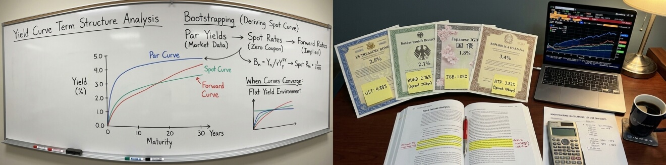
The yield curve is not a single line. Three distinct curves are used in fixed income analysis, each carrying different information.
The par curve shows the yields on hypothetical bonds priced at par, for each maturity. The spot curve (also called the zero-coupon curve) shows the yield on a single cash flow at each maturity, with no intermediate coupon payments. The forward curve shows the market’s implied yield for a loan beginning at a future date. The three curves diverge whenever the yield curve is not flat: in an upward-sloping environment, spot rates are above par rates at long maturities, and forward rates are above spot rates.
The spot curve is the more theoretically pure instrument for bond pricing: discounting each cash flow at its own maturity-specific rate, rather than applying a single yield, gives a more accurate present value. Bootstrapping the spot curve from observable par yields is standard practice in fixed income analysis.
The “risk-free” benchmark yield curve used in most textbooks is typically constructed from government bonds. But government bonds are not identically risk-free across countries. US Treasuries, German Bunds, Japanese JGBs, and Italian BTPs are all government bonds; they trade at different yields because markets assign them different default probabilities. Using a government yield curve as a risk-free benchmark incorporates the issuer’s sovereign risk into the discount rate. Textbooks often elide this. The distinction matters when comparing instruments across currencies or when a sovereign’s credit quality changes.
What Financial Models Assume, and What They Skip
Standard quantitative finance models rest on a set of assumptions about how prices behave. The assumptions are not arbitrary – they produce tractable mathematics and historically reasonable approximations. But they are assumptions, and each one fails under certain conditions. The 2008 financial crisis produced extensive documentation of which assumptions failed and when.
Standard assumption | What it implies | What 2008 revealed |
|---|---|---|
Log-normal return distribution | Extreme events are vanishingly rare | Tail events occurred far more often than the model predicted |
Constant volatility | Risk is stable and forecastable | Volatility spiked non-linearly; correlations moved to 1 across asset classes |
Liquid markets | Positions can be unwound at quoted prices | Bid-ask spreads collapsed; entire asset classes became untradeable |
Independent risk factors | Diversification reliably reduces portfolio risk | Previously uncorrelated assets fell together; diversification failed when most needed |
Nassim Taleb’s The Black Swan (2007) argued that financial return distributions have fat tails, extreme events are far more probable than Gaussian models predict. His framework distinguishes between “Mediocristan” (where averages dominate and extremes are rare, as in height distributions) and “Extremistan” (where single events can dominate the total, as in financial returns). The book was published a year before the crisis. Markets moved in 2008 by amounts that, under a normal distribution, should have occurred roughly once in the lifetime of the universe.
Emanuel Derman’s Models Behaving Badly (2011) approaches the problem from a practitioner’s perspective. Derman worked at Goldman Sachs developing the Black-Derman-Toy interest rate model and co-developing the Black-Scholes volatility smile. His argument is that financial models are metaphors, not laws: they describe behavior under certain conditions without capturing the underlying mechanism. Confusing a model for a law leads to applying it beyond its valid range. The Gaussian copula model used to price collateralised debt obligations was applied to instruments whose underlying correlations were not historically stable, and when housing prices fell nationally rather than locally, the model’s output became meaningless.
Where the Math Ends and Judgment Starts
A duration estimate tells you how sensitive a bond’s price is to a parallel shift in yield. It does not tell you whether that shift will occur, how large it will be, or whether the shift will in fact be parallel. A yield curve model tells you the market’s implied forward rates. It does not tell you whether those rates will be realised. Model output is an input to decision-making, not a decision.
The precision of quantitative output can imply more certainty than the underlying assumptions warrant. A bond priced to four decimal places using a sophisticated yield curve model has not been priced with four decimal places of accuracy. The precision reflects the calculation, not the estimate. The model’s assumptions about the discount rate, the shape of the yield curve, and the stability of credit spreads each carry uncertainty that is not reflected in the output’s decimal places.
Fixed income models are used to communicate risk – to compare instruments, to aggregate exposures, to set limits. A portfolio with modified duration 6.3 has a known sensitivity to rate moves under normal conditions. That number enables comparison and hedging. What it does not do is tell you when those conditions will cease to hold. Risk management uses models because the alternative is no common language for risk. The limitation is not a reason to avoid quantitative methods; it is a calibration note on what those methods deliver.